Chapter 1

1.1 A brief history of FV³

FV³ is a natural evolution of the hydrostatic Finite-Volume dynamical core (FV core) originally developed in the 90s on the latitude-longitude grid. The FV core started its life at NASA/Goddard Space Flight Center (GSFC) during early and mid 90s as an offline transport model with emphasis on the conservation, accuracy, consistency (tracer to tracer correlation), and efficiency of the transport process. The development and applications of monotonicity preserving Finite-Volume schemes at GSFC were motivated in part by the need to have a solution for the noisy and unphysical negative water vapor and chemical species (L94, LR96). It subsequently has been used by several high-profile Chemistry Transport Models (CTMs), including the NASA community GMI model (Rotman et al., 2001, J. Geophys. Res.), GOCART (Chin et al., 2000, J. Geophys. Res.), and the Harvard University-developed GEOS-CHEM community model (Bey et al, 2001, , J. Geophys. Res.). This transport module has also been used by some climate models, including the ECHAM5 AGCM (Roeckner et al, 2003, MPI-Report No. 349). Motivated by the success of monotonicity-preserving FV schemes in CTM applications, a consistently-formulated shallow-water model was developed. This solver was first presented at the 1994 PDE on the Sphere Workshop, and published in LR97. The Lin-Rood algorithm for shallow-water equations maintains mass conservation and a key Mimetic property of “no false vorticity generation”, and for the first time in computational geophysical fluid dynamics, uses high-order monotonic advection consistently for momentum and all other prognostic variables, instead of the inconsistent hybrid finite difference and finite-volume approach used by practically all other “finite volume” models today. The full 3D hydrostatic dynamical core, the FV core, was constructed based on the LR96 transport algorithm and the Lin-Rood shallow-water algorithm (LR97). The pressure gradient force is computed by the L97 finite-volume integration method, derived from Green’s integral theorem and based directly on first principles, and demonstrated errors an order of magnitude smaller than other pressure-gradient schemes at the time. The vertical discretization is the “vertically Lagrangian” scheme described by L04, the most powerful aspect of FV³, which permits great computational efficiency as well as greater accuracy given the same vertical resolution. The FV core was implemented in the NCAR CESM model in 2001 (Rasch et al, 2006, J. Climate) and in the GFDL CM2 model in 2004 (Delworth et al, 2006, J. Climate).

The need to scale to larger number of processors in modern massively parallel environments and the scientific advantage of eliminating the polar filter led to the development of FV³, the cubed-sphere version of FV. The cubed-sphere FV³ is in use in all GFDL and GSFC global models, and the cubed-sphere version of the LR96 advection scheme is used by the most recent version of GEOS-CHEM. Most recently, a computationally efficient non-hydrostatic solver has been implemented using a traditional semi-implicit approach for treating the vertically propagating sound waves. A second option for the non-hydrostatic solver, using a Riemann solver to nearly exactly solve for vertical sound-wave propagation, is also available. The Riemann solver is highly accurate and is very efficient if the Courant number for vertical sound wave propagation is small, and so may be very useful for extremely high (< 1 km) horizontal resolutions. In July 2016 this non-hydrostatic core has been selected for the Next-Generation Global Prediction System (NGGPS), paving the way for the unification of not only weather and climate models but also potentially regional and global models.

1.2 Outline of the solver

FV³ is the solver that integrates the compressible, adiabatic Euler equations in a weather or climate model. The solver is modular and designed to be called as a largely independent component of a numerical model, consistent with modern standards for model design; however for best results it is recommended that a model using FV³ as its dynamical core should use the provided application programming interface (API) to invoke the solver as well as to use the provided utility routines consistent with the dynamics, particularly for the initialization, updating the model state by time tendencies from the physics, and for incorporating increments from the data assimilation system.

The leftmost column of Figure 1.1 shows the external API calls used during a typical process-split model integration procedure. First, the solver is called, which advances the solver a full “physics” time step. This updated state is then passed to the physical parameterization package, which then computes the physics tendencies over the same time interval. Finally, the tendencies are then used to update the model state using a forward-in-time evaluation consistent with the dynamics, as described in Chapter 3.

There are two levels of time-stepping inside FV³. The first is the “remapping” loop, the orange column in Figure 1.1. This loop has three steps:

1. Perform the Lagrangian dynamics, the loop shown in the green column of Figure 1.1
2. Perform the sub-cycled tracer advection along Lagrangian surfaces,using accumulated mass fluxes from the Lagrangian dynamics. Subcycling is done independently within each layer to maintain local (within each layer) stability.
3. Remap the deformed Lagrangian surfaces on to the reference, or “Eulerian”, coordinate levels.

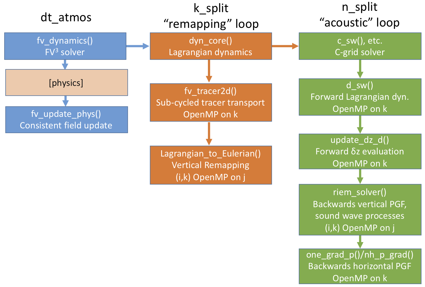
Figure 1.1: FV3 structure, including subroutines and time-stepping. Blue represents external API routines, called once per physics time step; orange routines are called once per remapping time step; green routines once per acoustic time step.

This loop is typically performed once per call to the solver, although it is possible to improve the model’s stability by executing the loop (and thereby the vertical remapping) multiple times per solver call.

The Lagrangian dynamics is the second level of time-stepping in FV³. This is the integration of the dynamics along the Lagrangian surfaces, across which there is no mass transport. Since the time step of the Lagrangian dynamics is limited by horizontal sound-wave processes, this is called the “acoustic” time step loop. (Note that the typical assumption that the advective wind speed is much slower than the sound wave speed is often violated near the poles, since the speed of the polar night jets can exceed two-thirds of the speed of sound.) The Lagrangian dynamics has two parts: the C-grid winds are advanced a half-time step, using simplified (but similarly constructed) core routines, which are then used to provide the advective fluxes to advance the D-grid prognostic fields a full time step. The integration procedure is similar for both grids: the along-surface flux terms (mass, heat, vertical momentum, and vorticity, and the kinetic energy gradient terms) are evaluated forward-in-time, and the pressure-gradient force and elastic terms are then evaluated backwards-in-time, to achieve enhanced stability.