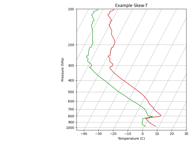
Creating a Skew-T Log-p Plot

EMCPy has a method to produce skew-T log-p plots. Given pressure, temperature, and dewpoint temperature data, users can call the SkewT() method to create a plot with the appropriate x and y axes.

import numpy as np
import matplotlib.pyplot as plt
from io import StringIO

from emcpy.plots.plots import SkewT
from emcpy.plots.create_plots import CreatePlot, CreateFigure


def _getSkewTData():
    # use data for skew-t log-p plot

    # Some example data.
    data_txt = '''
        978.0    345    7.8    0.8
        971.0    404    7.2    0.2
        946.7    610    5.2   -1.8
        944.0    634    5.0   -2.0
        925.0    798    3.4   -2.6
        911.8    914    2.4   -2.7
        906.0    966    2.0   -2.7
        877.9   1219    0.4   -3.2
        850.0   1478   -1.3   -3.7
        841.0   1563   -1.9   -3.8
        823.0   1736    1.4   -0.7
        813.6   1829    4.5    1.2
        809.0   1875    6.0    2.2
        798.0   1988    7.4   -0.6
        791.0   2061    7.6   -1.4
        783.9   2134    7.0   -1.7
        755.1   2438    4.8   -3.1
        727.3   2743    2.5   -4.4
        700.5   3048    0.2   -5.8
        700.0   3054    0.2   -5.8
        698.0   3077    0.0   -6.0
        687.0   3204   -0.1   -7.1
        648.9   3658   -3.2  -10.9
        631.0   3881   -4.7  -12.7
        600.7   4267   -6.4  -16.7
        592.0   4381   -6.9  -17.9
        577.6   4572   -8.1  -19.6
        555.3   4877  -10.0  -22.3
        536.0   5151  -11.7  -24.7
        533.8   5182  -11.9  -25.0
        500.0   5680  -15.9  -29.9
        472.3   6096  -19.7  -33.4
        453.0   6401  -22.4  -36.0
        400.0   7310  -30.7  -43.7
        399.7   7315  -30.8  -43.8
        387.0   7543  -33.1  -46.1
        382.7   7620  -33.8  -46.8
        342.0   8398  -40.5  -53.5
        320.4   8839  -43.7  -56.7
        318.0   8890  -44.1  -57.1
        310.0   9060  -44.7  -58.7
        306.1   9144  -43.9  -57.9
        305.0   9169  -43.7  -57.7
        300.0   9280  -43.5  -57.5
        292.0   9462  -43.7  -58.7
        276.0   9838  -47.1  -62.1
        264.0  10132  -47.5  -62.5
        251.0  10464  -49.7  -64.7
        250.0  10490  -49.7  -64.7
        247.0  10569  -48.7  -63.7
        244.0  10649  -48.9  -63.9
        243.3  10668  -48.9  -63.9
        220.0  11327  -50.3  -65.3
        212.0  11569  -50.5  -65.5
        210.0  11631  -49.7  -64.7
        200.0  11950  -49.9  -64.9
        194.0  12149  -49.9  -64.9
        183.0  12529  -51.3  -66.3
        164.0  13233  -55.3  -68.3
        152.0  13716  -56.5  -69.5
        150.0  13800  -57.1  -70.1
        136.0  14414  -60.5  -72.5
        132.0  14600  -60.1  -72.1
        131.4  14630  -60.2  -72.2
        128.0  14792  -60.9  -72.9
        125.0  14939  -60.1  -72.1
        119.0  15240  -62.2  -73.8
        112.0  15616  -64.9  -75.9
        108.0  15838  -64.1  -75.1
        107.8  15850  -64.1  -75.1
        105.0  16010  -64.7  -75.7
        103.0  16128  -62.9  -73.9
        100.0  16310  -62.5  -73.5
    '''

    # Parse the data
    sound_data = StringIO(data_txt)
    p, h, T, Td = np.loadtxt(sound_data, unpack=True)

    return p, T, Td


def main():

    p, T, Td = _getSkewTData()

    tplot = SkewT(T, p)
    tplot.color = 'tab:red'

    tdplot = SkewT(Td, p)
    tdplot.color = 'tab:green'

    plot1 = CreatePlot()
    plot1.plot_layers = [tplot, tdplot]
    plot1.add_grid()
    plot1.add_xlabel('Temperature (C)')
    plot1.add_ylabel('Pressure (hPa)')
    plot1.add_title('Example Skew-T')

    fig = CreateFigure()
    fig.plot_list = [plot1]
    fig.create_figure()
    fig.tight_layout()

    plt.show()


if __name__ == '__main__':
    main()