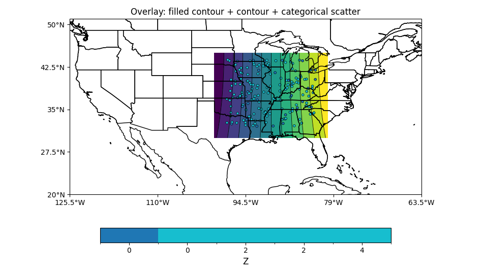
Overlay: filled contour + contour + scatter

Demonstrates layering multiple EMCPy map types.

import numpy as np
from emcpy.plots.map_plots import MapFilledContour, MapContour, MapScatter
from emcpy.plots.create_plots import CreatePlot, CreateFigure

# Field (centers)
lon = np.linspace(-100, -80, 121)
lat = np.linspace(30, 45, 91)
LON, LAT = np.meshgrid(lon, lat)
Z = np.cos(np.radians(LON)) * np.sin(np.radians(LAT * 2))

# Random stations
rng = np.random.default_rng(2)
n = 180
slat = rng.uniform(32, 44, n)
slon = rng.uniform(-98, -82, n)
cat = rng.integers(0, 5, n)   # categories for scatter

p = CreatePlot(projection="plcarr", domain="conus")

# 1) Filled background
cf = MapFilledContour(LAT, LON, Z)
cf.cmap = "viridis"
cf.levels = np.linspace(Z.min(), Z.max(), 13)

# 2) Thin contour lines
c = MapContour(LAT, LON, Z)
c.levels = np.linspace(Z.min(), Z.max(), 13)
c.colors = "black"
c.linewidths = 0.6

# 3) Categorical scatter on top
ms = MapScatter(slat, slon, data=cat)
ms.integer_field = True
ms.cmap = "tab10"
ms.markersize = 12
ms.edgecolors = "k"
ms.linewidths = 0.5

p.plot_layers = [cf, c, ms]
p.add_map_features(["states", "coastline"])
p.add_colorbar(label="Z")
p.add_title("Overlay: filled contour + contour + categorical scatter")

fig = CreateFigure(1, 1, figsize=(9.5, 5.4))
fig.plot_list = [p]
fig.create_figure()
fig.tight_layout()